SQL versus R - who is faster?

225 lines of code (R)

Is it worth organising your data in a data base if all you are interested in is speed? It depends on what you are doing with the data. This guide teaches you where to expect speed advantages of SQLite and R.

Set up

Organising your data in a data base brings many advantages. Few people probably think of speed as an issue. Usually memory and stability issues come up way before. This made me wonder, if you want to optimise your code for speed, is SQL beneficial?

In this little tutorial I will compare SQLite and R without any additional libraries (base R). Thanks to the RSQLite library this can all be done in the same R session. We start off by loading libraries for benchmarking (assessing performance of code snippets), SQL, and plotting.

library(microbenchmark)
library(RSQLite)
library(DBI)
library(ggthemes)
library(ggplot2)

Next, we initialise the data bases: db_disk is a temporary data base on disk while db_mem resides in memory.

db_disk <- dbConnect(RSQLite::SQLite(), "")#tmp
db_mem <- dbConnect(RSQLite::SQLite(), "file::memory:")

We populate the data bases with a single table which most R users will be very familiar with: the iris data set. It includes five columns, four of which are numerical, and 150 rows.

dbWriteTable(db_disk, "iris", iris)
dbWriteTable(db_mem, "iris", iris)

We wrap up the set-up with functions fun_disk() and fun_mem() which we will benchmark. The result will be plotted as a minimalist Tufte style box plot by fun_plot().

fun_disk <- function(query, db_disk. = db_disk) dbGetQuery(db_disk., query)
fun_mem <- function(query, db_mem. = db_mem) dbGetQuery(db_mem., query)

fun_plot <- function(dat_box=tm, y_lim = c(10, 50000)){

  dat_box$time = dat_box$time/1000

  A = ggplot(dat_box, aes(x = expr, group = expr, y = time)) +
    geom_tufteboxplot(median.type = "line", whisker.type = 'line', hoffset = 0, width = 3) +
    xlab("") +
    ylab("Execution Time (microseconds)") +
    scale_y_log10(limits = y_lim, breaks = 10^(1:4)) +
    scale_x_discrete(labels = c("SQL\non disk",
                                "SQL\nin memory",
                                "base R\nin memory\n(variation 1)",
                                "base R\nin memory\n(variation 2)")) +
    theme_tufte(ticks = F) +
    theme(axis.text.x = element_text(size=12)) +
    labs(caption = '@rikunert') +
    theme(plot.caption = element_text(size = 10, color = 'grey', face= 'italic'))

  A  
}

In the following we will compare the performance of these two data bases with equivalent operations in R. Each time, I’ll come up with two different ways of getting to the same result in R.

Basic query

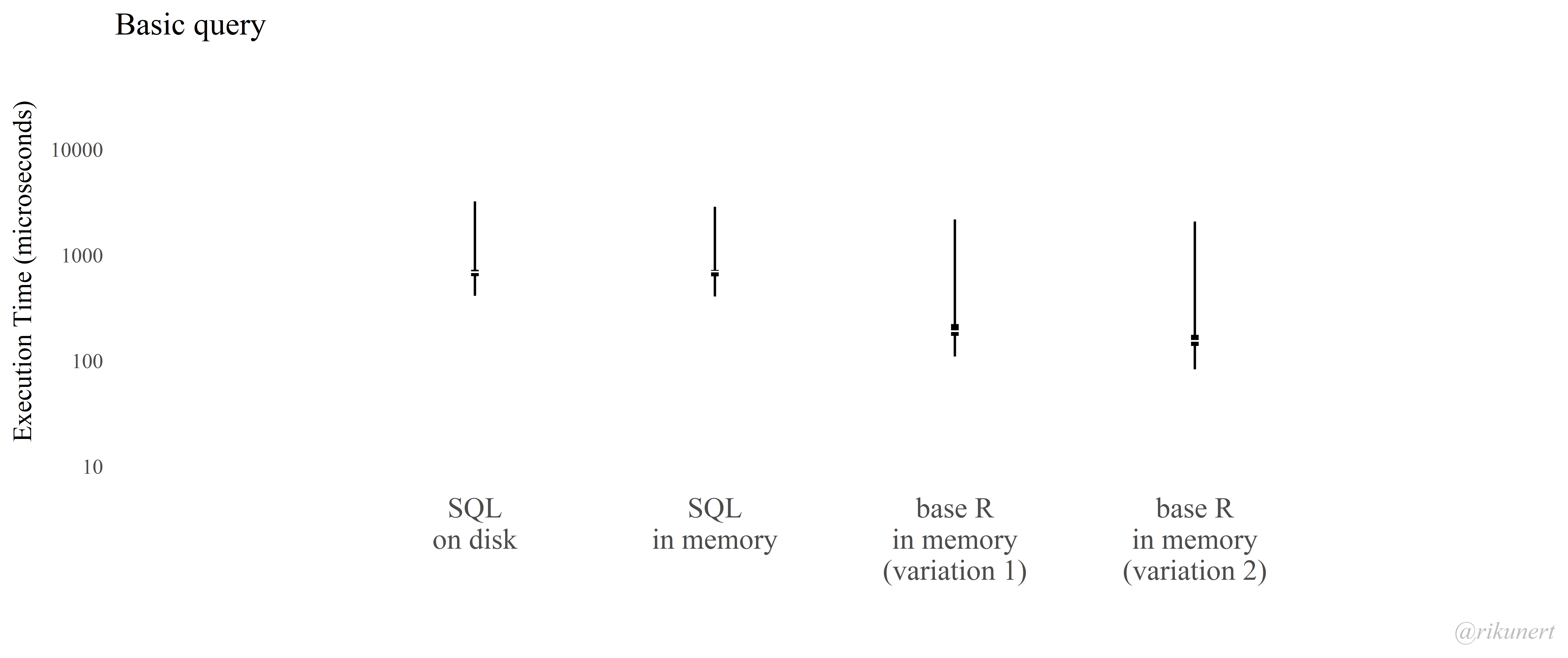
We begin the tests with a simple query which just displays the first 5 rows and all columns. Turns out that R can do that a lot faster at 200 - 300 microseconds compared to around 1000 microseconds for SQL.

You can re-create this analysis and figure by running the following code. All other examples will follow this example in structure. Write the SQL query for the data base. Note that it is conventional in SQL to write variables with small letters and all else with big letters.

query = 'SELECT * FROM iris LIMIT 5'

Define two functions getting to the same result as the query but through R via two different routes.

fun_base1 <- function(data = iris) head(data, 5)
fun_base2 <- function(data = iris) data[1:5,]

Perform the benchmarking of the four functions. Two functions for SQL, and two for base R. The result is stored in tm.

tm = microbenchmark(fun_disk(query), fun_mem(query), fun_base1(), fun_base2())

Plot the result and save with dimensions optimised for social media (1240 x 520).

fun_plot(dat_box = tm) + ggtitle('Basic query')
ggsave('SQL_R_bench_1.png',width = 12.9, height = 5.42, scale = 0.7, dpi = 1000)

Out of interest, have a look what the result of the query actually is.

dbGetQuery(db_mem, query)

Aggregation & grouping

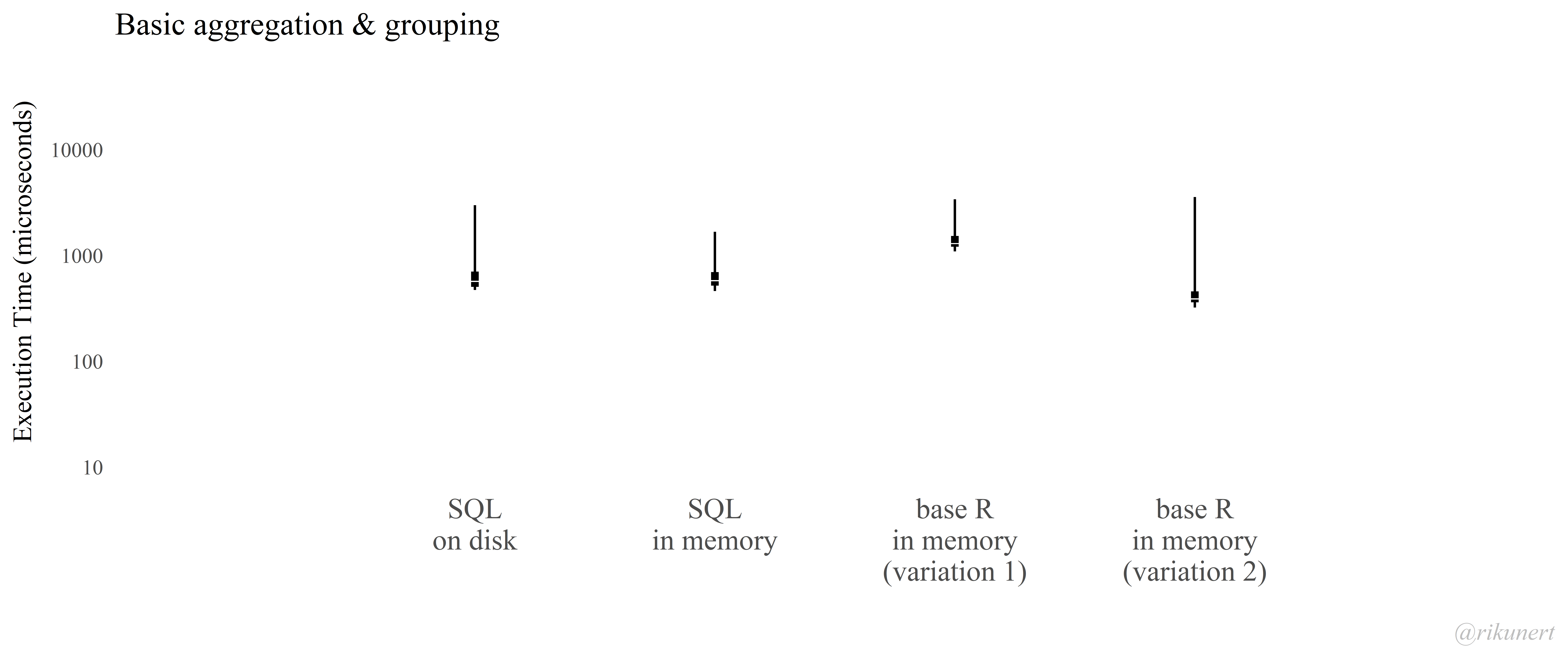
How about simple aggregation, i.e. the summary of values? In this example I look at the mean, or AVG() in SQL. To spice things up somewhat I aggregate based on a categorical variable. So, I look for the average petal length of different iris species.

Here, SQL performs well at around 750 microseconds. R needs more or less time depending on whether one uses the aggregate() function (1600 microseconds) or the by() function (450 microseconds).

query = 'SELECT species, AVG("Petal.Length") FROM iris GROUP BY species'
fun_base1 <- function(data = iris) aggregate(data$Petal.Length~data$Species, FUN=mean)
fun_base2 <- function(data = iris) by(data$Petal.Length, data$Species, mean)

tm = microbenchmark(fun_disk(query), fun_mem(query), fun_base1(), fun_base2())

fun_plot(dat_box = tm) + ggtitle('Basic aggregation')
ggsave('SQL_R_bench_2.png',width = 12.9, height = 5.42, scale = 0.7, dpi = 1000)

dbGetQuery(db_mem, query)

Aggregation & conditional

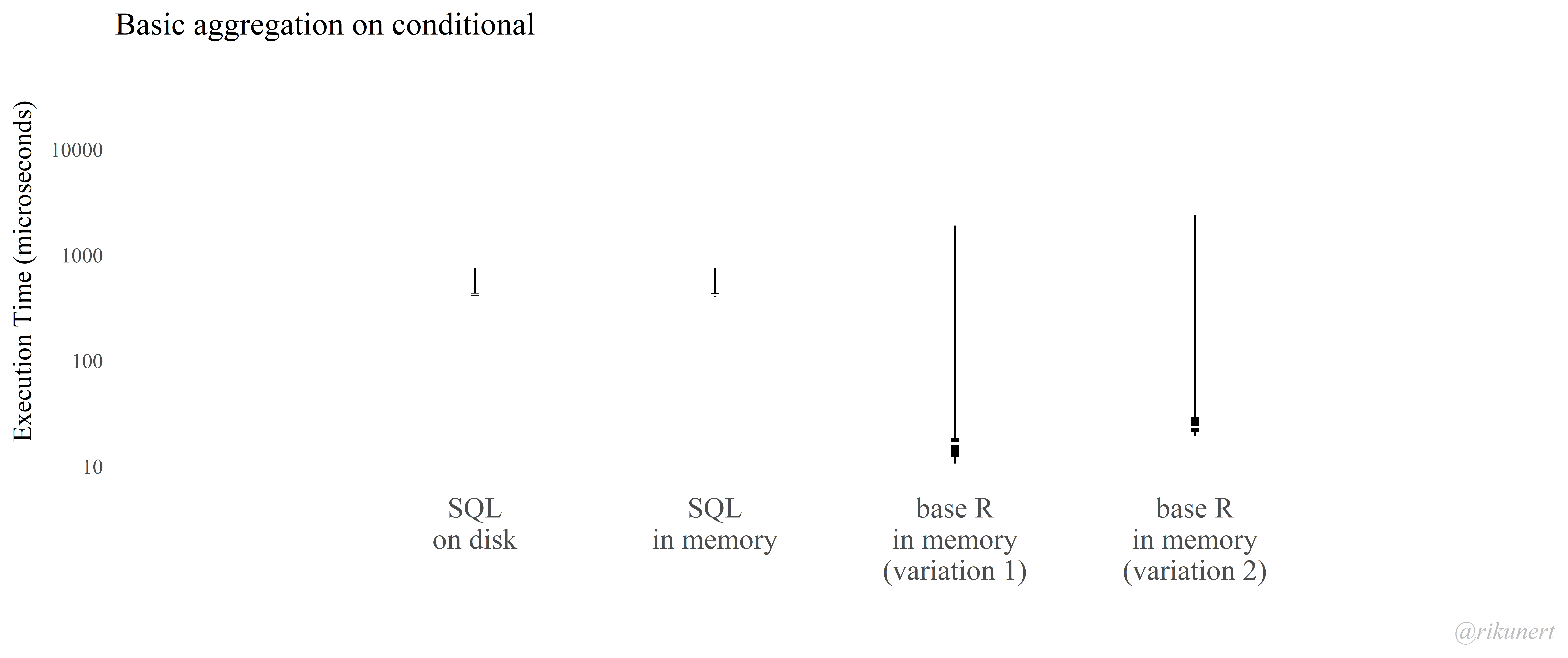
And if the aggregation uses a different function, COUNT() in this case, and a conditional (if else in most programming languages but not in SQL)? In this example I ask how many individal flowers (rows) have a petal length greater than or equalling 2.

Here, SQL performs at its usual pace at 915 microseconds while R shows off its speed at 25 - 55 microseconds.

query = 'SELECT species, COUNT(*) FROM iris WHERE "Petal.Length" >= 2'
fun_base1 <- function(data = iris) sum(data$Petal.Length > 2)
fun_base2 <- function(data = iris) length(data$Petal.Length[data$Petal.Length > 2])

tm = microbenchmark(fun_disk(query), fun_mem(query), fun_base1(), fun_base2())

fun_plot(dat_box = tm) + ggtitle('Basic aggregation on conditional')
ggsave('SQL_R_bench_3.png',width = 12.9, height = 5.42, scale = 0.7, dpi = 1000)

dbGetQuery(db_mem, query)

Temporary variable & aggregation & condition

Having covered the basics, it is time to get into slightly more advanced territory. What if we construct a temporary variable size (which codes petal length as either small, intermediate, or big)? We can then aggregate based on two grouping variables species and size. In essence, I am asking how many individuals of each iris species had small, intermediate, and large petals.

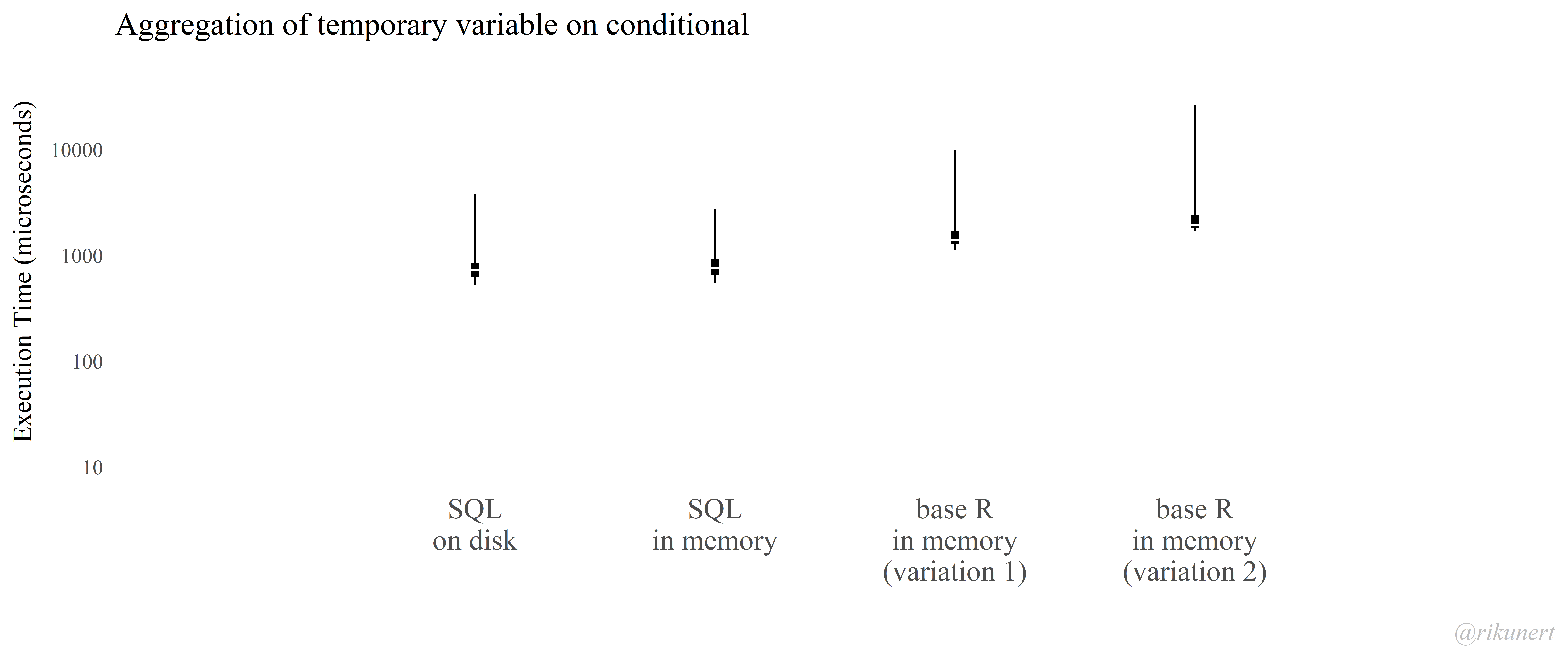
This question is answered the fastest by SQL at 815 microseconds. R needs a lot longer. It needs 1400 microseconds if one constructs a temporary variable species and then uses the aggregate() function to get the desired result, see fun_base1(). Things take even longer (2100 microseconds) if one loops over species and sums petal lengths without a temporary variable species, see fun_base2().

query = 'SELECT species,
CASE  
WHEN "Petal.Length" < 2 THEN \'small\'
WHEN "Petal.Length" > 5 THEN \'big\'
ELSE \'intermediate\'
END AS size,
COUNT(*)
FROM iris
GROUP BY 1, 2;'

fun_base1 <- function(data = iris) {
  size = rep('intermediate', nrow(data))
  size[data$Petal.Length < 2] = 'small'
  size[data$Petal.Length > 5] = 'big'
  aggregate(rep(1, nrow(data)),#just a vector of 1s which will get added up
            by=list(Species = data$Species, size = size),
            FUN=sum)
}

fun_base2 <- function(data = iris) {
  out = data.frame(Species = rep(unique(data$Species), each = 3),
                   size = rep(c('big', 'intermediate', 'small'), 3),
                   count = rep(NA, 3*3))
  for (Species in unique(data$Species)){
    out$count[out$Species == Species & out$size == 'small'] = sum(data$Species == Species & data$Petal.Length < 2)
    out$count[out$Species == Species & out$size == 'intermediate'] = sum(data$Species == Species & data$Petal.Length >= 2 & data$Petal.Length <= 5)
    out$count[out$Species == Species & out$size == 'big'] = sum(data$Species == Species & data$Petal.Length > 5)
  }
}

tm = microbenchmark(fun_disk(query), fun_mem(query), fun_base1(), fun_base2())

fun_plot(dat_box = tm) + ggtitle('Aggregation of temporary variable on conditional')
ggsave('SQL_R_bench_4.png',width = 12.9, height = 5.42, scale = 0.7, dpi = 1000)

dbGetQuery(db_mem, query)

Create table and add to data base

Beyond creating a temporary variable just for one query, one can of course also add a new table to a data base. I looked up the blooming months of different iris species and summarise them in the table flowers. How long does it take to add this to the data base?

Unfortunately, one has to split this task in three for SQL. First, we check whether the table flowers already exists and if so delete it. Next, we initialise a new table flowers with three columns. Finally, we populate the table with data for four iris species. This information was taken from wikipedia. Note that because we don’t query the data bases for returned data, we don’t use dbGetQuery() but instead dbExecute().

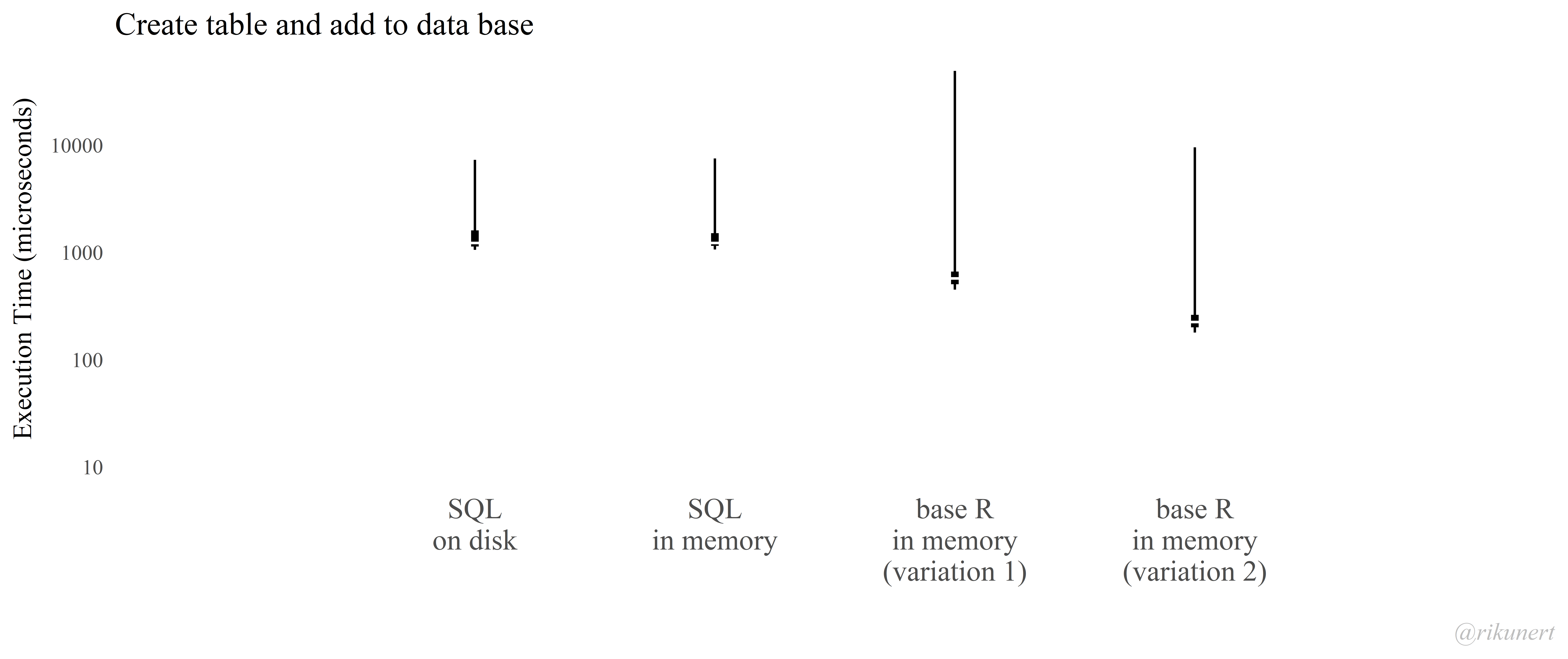
In R, we either just create a basic data frame or go a rather more convoluted route and first create a matrix which we then turn into a data frame. To my own surprise, the latter approach was the fastest at 250 microseconds. The straight forward data frame approach took much longer at 850 microseconds. SQL was the slowest at around 1300 microseconds.

query1 = 'DROP TABLE IF EXISTS flowers;'
query2 = 'CREATE TABLE flowers (species TEXT, bloom_start TEXT, bloom_end TEXT);'
query3 = 'INSERT INTO flowers (species, bloom_start, bloom_end)
VALUES
(\'setosa\', \'June\', \'July\'),
(\'versicolor\', \'May\', \'July\'),
(\'virginica\', \'April\', \'May\'),
(\'pallida\', \'May\', \'June\');'

fun_disk_exe3 <- function(statements, db_disk. = db_disk) lapply(1:3, function(x) dbExecute(db_disk., statements[x]))
fun_mem_exe3 <- function(statements, db_mem. = db_mem) lapply(1:3, function(x) dbExecute(db_mem., statements[x]))

fun_base1 <- function(data = iris) {
  flowers = data.frame(species = c('setosa', 'versicolor', 'virginica', 'pallida'),
                       bloom_start = c('June', 'May', 'April', 'May'),
                       bloom_end = c('July', 'July', 'May', 'June'))
}

fun_base2 <- function(data = iris) {
  flowers = rbind(c('setosa','June','July'),
                  c('versicolor', 'May', 'July'),
                  c('virginica', 'April', 'May'),
                  c('pallida', 'May', 'June')
                  )
  colnames(flowers) = c('species', 'bloom_start', 'bloom_end')
  as.data.frame(flowers)
}

tm = microbenchmark(fun_disk_exe3(c(query1, query2, query3)), fun_mem_exe3(c(query1, query2, query3)), fun_base1(), fun_base2())

fun_plot(dat_box = tm) + ggtitle('Create table and add to data base')
ggsave('SQL_R_bench_5.png',width = 12.9, height = 5.42, scale = 0.7, dpi = 1000)

Joining 2 tables

Having constructed both tables, how long does it take to join them? Joining two tables basically boils down to extending the rows of one table by the columns of another table. The right rows of one table need to be matched with the right rows of another table. In SQL the matching variable resides in a column which JOIN ON calls, in this case species.

Turns out R has a neat function which does that in one go, called merge(). An alternative approach, implemented in fun_base1(), would be to go through one table line by line and do the matching with a loop.

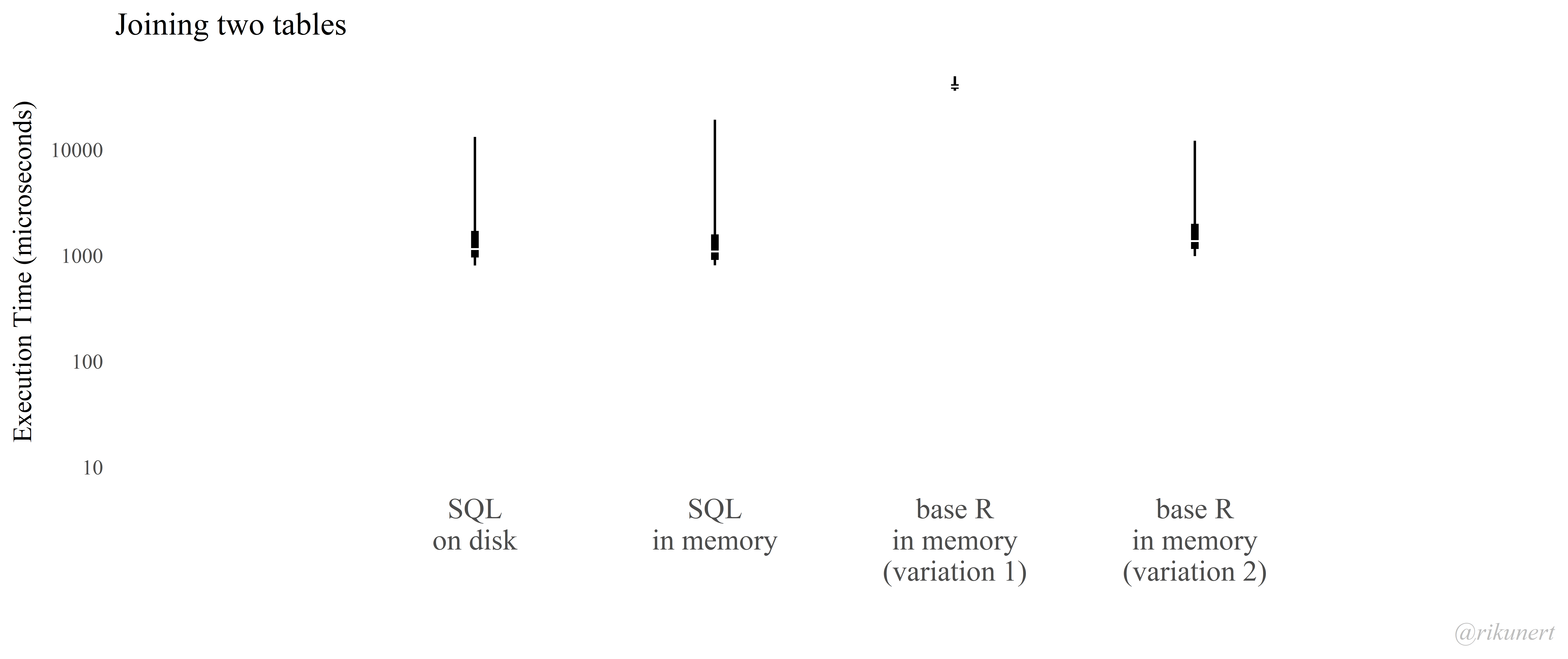
Perhaps unsurprisingly, the loop is the slowest approach at 48200 microseconds. merge() performs much better at 1350 microseconds. However, SQL clearly beats R in this contest at around 1200 microseconds.

For the code in this example to work you need to have included the second table flowers in the data bases, as shown in the previous step.

query = 'SELECT * FROM flowers
JOIN iris ON
flowers.species = iris.species'

flowers = data.frame(species = c('setosa', 'versicolor', 'virginica', 'pallida'),
                     bloom_start = c('June', 'May', 'April', 'May'),
                     bloom_end = c('July', 'July', 'May', 'June'))

fun_base1 <- function(data1 = iris, data2 = flowers) {
  data1$bloom_start = NA
  data1$bloom_end = NA
  for(i in 1:dim(data1)[1]){#for each row in data1
    data1[i, 6] = as.character(data2[data2$species == as.character(data1$Species[i]), 2])
    data1[i, 7] = as.character(data2[data2$species == as.character(data1$Species[i]), 3])
  }
  return(data1)
}

fun_base2 <- function(data1 = iris, data2 = flowers) {
  merge(data1, data2, by.x = 'Species', by.y = 'species')
}

tm = microbenchmark(fun_disk(query), fun_mem(query), fun_base1(), fun_base2())

fun_plot(dat_box = tm) + ggtitle('Joining two tables')
ggsave('SQL_R_bench_6.png',width = 12.9, height = 5.42, scale = 0.7, dpi = 1000)

dbGetQuery(db_disk, query)

Joining 2 tables, aggregation, & grouping

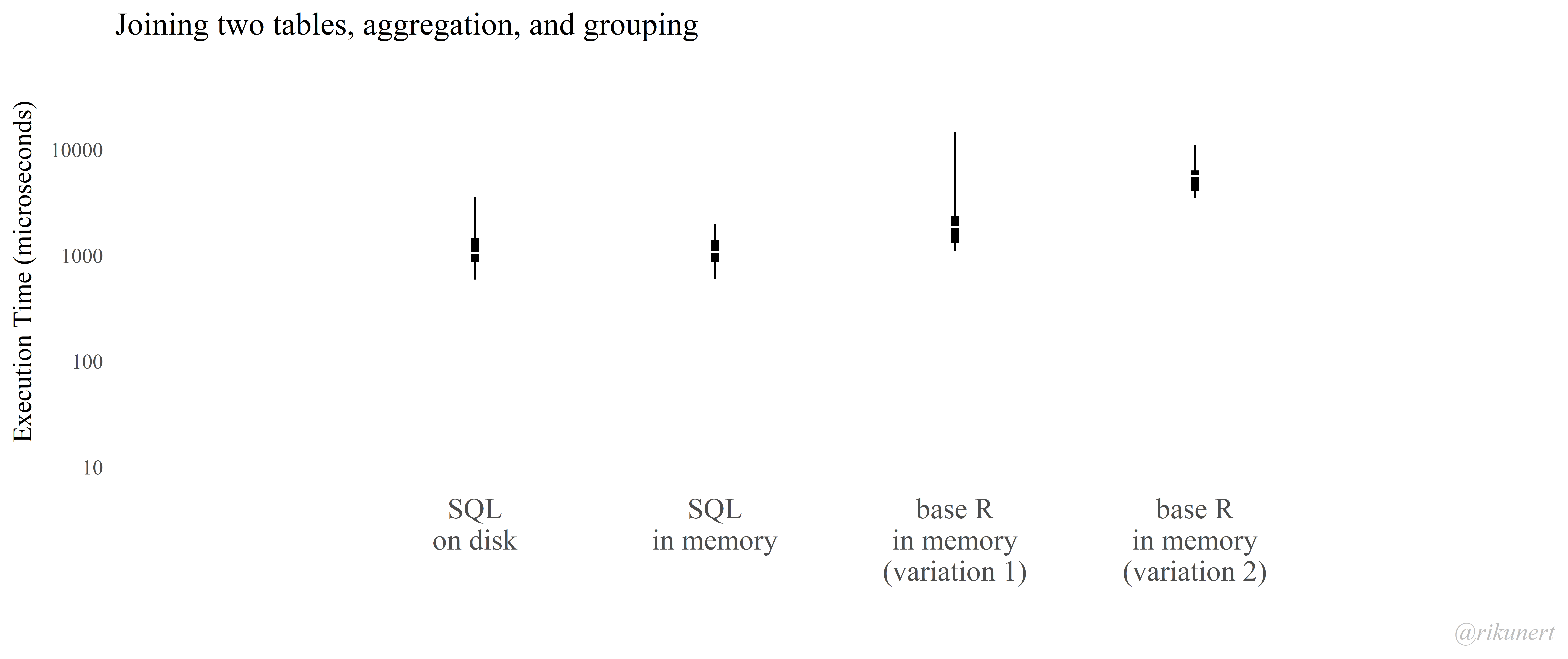
Let’s use a lot of functions which we encountered so far and see how their combination changes performance. In this last test we join the iris and flowers tables and then look for the average petal length of species organised by the end of their flowering.

This can either be done via the for loop in fun_base1() or more elegantly with merge() and aggregate() as shown in fun_base2(). However, neither approach in R is fast. The first needs 1450 microseconds while the second needs 4180 microseconds. SQL gets there a lot faster at 880 microseconds.

query = 'SELECT flowers.bloom_end, AVG(iris."petal.length") FROM flowers
JOIN iris ON
flowers.species = iris.species
GROUP BY flowers.bloom_end'

fun_base1 <- function(data1 = iris, data2 = flowers) {
  out = matrix(rep(NA, length(unique(data2$bloom_end)) * 2), nrow = length(unique(data2$bloom_end)), ncol = 2)
  for (i in 1:length(unique(data2$bloom_end))){
    out[i,] = c(as.character(unique(data2$bloom_end)[i]),
            mean(data1$Petal.Length[
              grepl(paste(data2$species[data2$bloom_end == unique(data2$bloom_end)[i]],collapse = '|'),
                    data1$Species)]))
  }
}

fun_base2 <- function(data1 = iris, data2 = flowers) {
  x = merge(data1, data2, by.x = 'Species', by.y = 'species')
  aggregate(x = x, by=list(x$bloom_end), FUN=mean)[,c(1, 5)]
}

tm = microbenchmark(fun_disk(query), fun_mem(query), fun_base1(), fun_base2())

fun_plot(dat_box = tm) + ggtitle('Joining two tables and aggregation')
ggsave('SQL_R_bench_7.png',width = 12.9, height = 5.42, scale = 0.7, dpi = 1000)

dbGetQuery(db_disk, query)

Conclusion

Two things are noteworthy about the speed comparison between SQL and R.

First, while R performs some things with lightning speed and some other things quite slowly, SQL shows a remarkably stable performance at 750 to 1300 microseconds. This stable speed performance is not influenced by whether the data base resides on disk or in memory. So, dealing with data bases via SQL is not just stable in terms of data storage and access but also in terms of speed. R can get slow with more complicated queries while SQL keeps on performing well.

Second, the interested reader should keep some limitations of this comparison in mind:

• I work with a particular system and performance might vary between systems. I use a Lenovo L530 (windows 10, R version 3.4.0).
• The R-code I used can probably be made faster. I just wrote standard code, not speedy code.
• The data base I used was tiny. I have no idea whether the same conclusions hold for bigger data sets.
• The R-code I used here only worked with data in memory. Loading from and saving to disk takes additional time. This is not factored in. One SQL approach I benchmark interacts directly with disk.

Like this post? Share it with your followers or follow me on Twitter!